How we can predict stock price movements using Twitter
Note from Towards Data Science’s editors: While we allow independent authors to publish articles in accordance with our rules and guidelines, we do not endorse each author’s contribution. You should not rely on an author’s works without seeking professional advice. See our Reader Terms for details.
Do the markets reflect rational behavior or human irrationality? Mass psychology's effects may not be the only factor driving the markets, but it’s unquestionably significant [1].
This fascinating quality is something that we can measure and use to predict market movement with surprising accuracy levels.
With the real-time information available to us on massive social media platforms like Twitter, we have all the data we could ever need to create these predictions.
But then comes the question, how can our computer understand what this unstructured text data means? That is where sentiment analysis comes in. Sentiment analysis is a particularly interesting branch of Natural Language Processing (NLP), which is used to rate the language used in a body of text.
Through sentiment analysis, we can take thousands of tweets about a company and judge whether they are generally positive or negative (the sentiment) in real-time! We will cover:
> Getting Twitter Developer Access
  - API Setup

> Twitter API
  - Searching for Tweets
  - Improving our Request

> Building Our Dataset

> Sentiment Analysis
  - Flair
  - Analyzing Tesla Tweets

> Historical Performance
  - TSLA Tweets
  - TSLA Ticker
If you’re here for sentiment analysis in Flair — I cover it more succinctly in this video:
Getting Twitter Developer Access
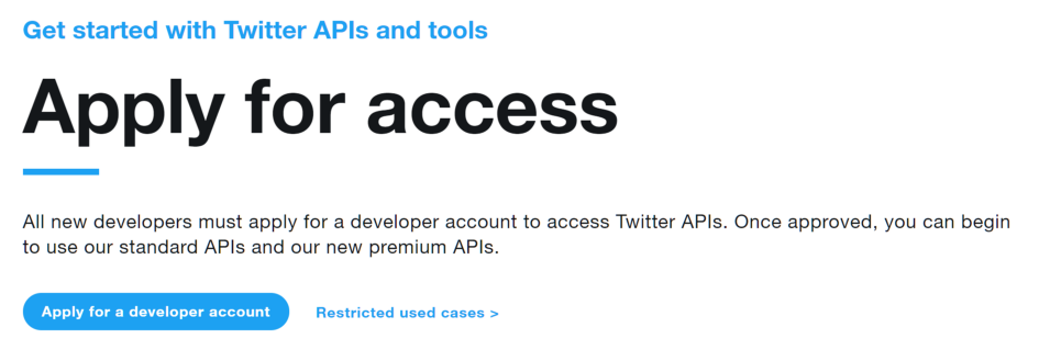
The very first thing we need to apply for Twitter developer access. We can do this by heading over to dev.twitter.com and clicking the Apply button (top-right corner).
On the next page, we click the ‘Apply for a developer account’ button; now, Twitter will ask us a few questions. Answer all of the questions as best you can.
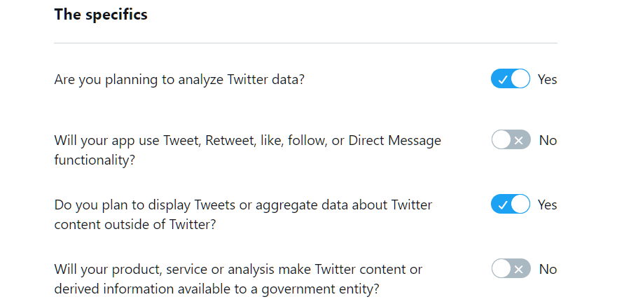
On the ‘How will you use the Twitter API or Twitter data?’ page, select yes or no, as shown above. I have put a few example answers here — these are only valid for this specific use-case, so please adjust them to your own needs where relevant.
We submit our answers and complete the final agreement and verification steps. Once complete, we should find ourselves at the app registration screen.
App Setup
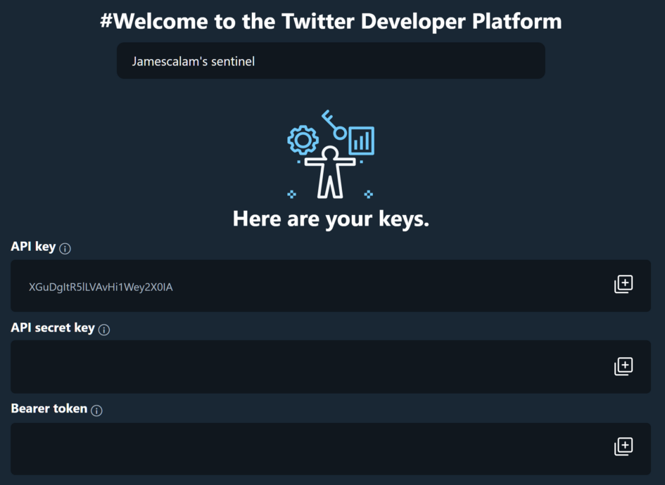
First, we give our app a name. It has to be unique, so be creative. We will receive our API keys; this is the only time we will see them, so keep them somewhere safe (and secret)!
Twitter API
Now we have our API set up; we can begin pulling tweet data. We will focus on Tesla for this article.
Searching for Tweets
We will be using the requests library to interact with the Twitter API. We can search for the most recent tweets given a query through the /tweets/search/recent endpoint.
Together with the Twitter API address, this gives us:
We need two more parts before sending our request, (1) authorization and (2) a search query. The bearer token given to us earlier is used for authorization — which we pass through the authorization key in our request header.
Finally, we can specify our search query by adding ?q=<SEARCH QUERY> to our API address. Putting these all together in a search for Telsa will give us:
requests.get(
    'https://api.twitter.com/1.1/search/tweets.json?q=tesla',
    headers={
 'authorization': 'Bearer '+BEARER_TOKEN
})
Improving Our Request
Our request will not return exactly what we want. If we take a look at the very first entry of our returned request we will see very quickly that we are not returning the full length of tweets — and that they may not even be relevant:
Fortunately, we can easily fix the tweet truncation by adding another parameter tweet_mode=extended to our request. Which will look like:
/search/tweets.json?q=tesla&tweet_mode=extendedAs we add more and more parameters, the API address string can quickly get overcrowded and messy. To avoid this, we can move them into a dictionary — which we then feed to the params argument of our get request.
params = {'q': 'tesla'
          'tweet_mode': 'extended'}requests.get(
    'https://api.twitter.com/1.1/search/tweets.json',
 params=params,
    headers={'authorization': 'Bearer '+BEARER_TOKEN}
})
We can improve our request further. First, we can tell Twitter which language tweets to return (otherwise we get everything) with lang=en for English. Adding count=100 increases the maximum number of tweets to return to 100.
params = {
    'q': 'tesla',
    'tweet_mode': 'extended',
    'lang': 'en',
    'count': '100'
}
Building Our Dataset
Once we have our API request setup, we can begin running it to populate our dataset.
def get_data(tweet):
    data = {
        'id': tweet['id_str'],
        'created_at': tweet['created_at'],
        'text': tweet['full_text']
    }
    return data
Each tweet returned by the API contains just three fields that we want to keep. Those are the tweet ID 'id_str', creation date 'created_at', and untruncated text 'full_text'. We extract these in a function called get_data.
Our response is not just one tweet — it contains many. So we need to iterate through each of these and extract the information we need.
df = pd.DataFrame()for tweet in response.json()['statuses']:
 row = get_data(tweet)
    df = df.append(row, ignore_index=True)
We first transform the API response into a Python dictionary using .json() — we then access the list of tweets through ['statuses']. We then extract tweet data with get_data and append to our dataframe df. Giving us:
Sentiment Analysis
We will be using a pre-trained sentiment analysis model from the flair library. As far as pre-trained models go, this is one of the most powerful.
This model splits the text into character-level tokens and uses the DistilBERT model to make predictions. The advantage of working at the character-level (as opposed to word-level) is that words that the network has never seen before can still be assigned a sentiment.
DistilBERT is a distilled version of the powerful BERT transformer model — which in-short means — it is a ‘small’ model (only 66 million parameters) AND is still super powerful [2].
Flair
To use the flair model, we first need to import the library with pip install flair. Once installed, we import and initialize the model like so:
import flair
sentiment_model = flair.models.TextClassifier.load('en-sentiment')
If you have issues installing Flair, it is likely due to your PyTorch/Tensorflow installations. For PyTorch, go here to get the correct installation command — and for Tensorflow type pip install tensorflow (add -U at the end to upgrade).
All we need to do now is tokenize our text by passing it through flair.data.Sentence(<TEXT HERE>) and calling the .predict method on our model. Putting those together, we get:
sentence = flair.data.Sentence(TEXT)
sentiment_model.predict(sentence)
By calling the predict method we add the sentiment rating to the data stored in sentence. We can see how it works by predicting the sentiment for a simple phrase:
And let’s try something negative:
It works on our two easy test cases, but we don’t know about actual tweets — which involve special characters and more complex language.
Analyzing Tesla Tweets
Most of our tweets are very messy. Cleaning text data is fundamental, although we will just do the bare minimum in this example.
whitespace = re.compile(r"\s+")
web_address = re.compile(r"(?i)http(s):\/\/[a-z0-9.~_\-\/]+")
tesla = re.compile(r"(?i)@Tesla(?=\b)")
user = re.compile(r"(?i)@[a-z0-9_]+")

# we then use the sub method to replace anything matching
tweet = whitespace.sub(' ', tweet)
tweet = web_address.sub('', tweet)
tweet = tesla.sub('Tesla', tweet)
tweet = user.sub('', tweet)
Using regular expressions (RegEx) through the re module, we can quickly identify excessive whitespace, web addresses, and Twitter users. If these expressions look like hieroglyphs to you — I covered all of these methods in a RegEx article here.
Now we have our clean(ish) tweet — we can tokenize it by converting it into a sentence object, and then predict the sentiment:
sentence = flair.data.Sentence(tweet)
sentiment_model.predict(sentence)
Finally, we extract our predictions and add them to our tweets dataframe. We can access the label object (the prediction) by typing sentence.labels[0]. With this, we call score to get our confidence/probability score, and value for the POSITIVE/NEGATIVE prediction:
probability = sentence.labels[0].score  # numerical value 0-1
sentiment = sentence.labels[0].value  # 'POSITIVE' or 'NEGATIVE'
We can append the probability and sentiment to lists which we then merge with our tweets dataframe. Putting all of these parts together will give us:
# we will append probability and sentiment preds later
probs = []
sentiments = []

# use regex expressions (in clean function) to clean tweets
tweets['text'] = tweets['text'].apply(clean)

for tweet in tweets['text'].to_list():
    # make prediction
    sentence = flair.data.Sentence(tweet)
    sentiment_model.predict(sentence)
    # extract sentiment prediction
    probs.append(sentence.labels[0].score)  # numerical score 0-1
    sentiments.append(sentence.labels[0].value)  # 'POSITIVE' or 'NEGATIVE'

# add probability and sentiment predictions to tweets dataframe
tweets['probability'] = probs
tweets['sentiment'] = sentiments
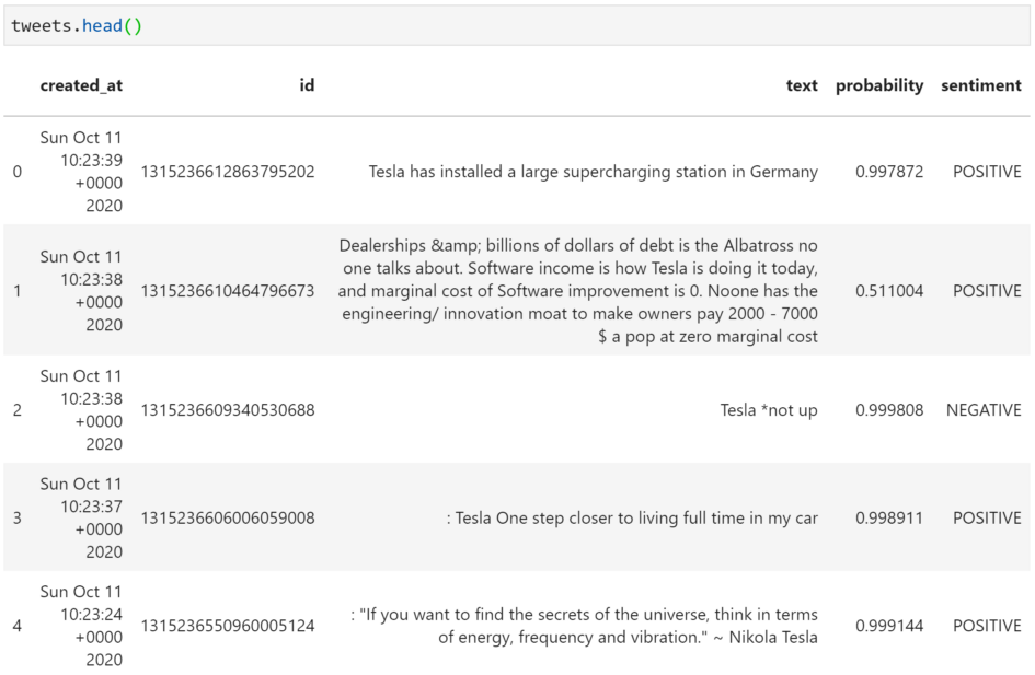
A quick look at the head of our dataframe shows some pretty impressive results. The second tweet is assigned a positive sentiment, but with a low level of confidence (0.51) — as a human, I’m also not sure whether this is a positive or negative tweet either.
Tweet number three, “Tesla *not up”, demonstrates how effective using character-level embeddings can be.
With word embeddings, it is improbable that our model would recognize ‘*not’ as matching the word ‘not’. Our character-level model doesn’t trip up and accurately classifies the tweet as negative.
Historical Performance
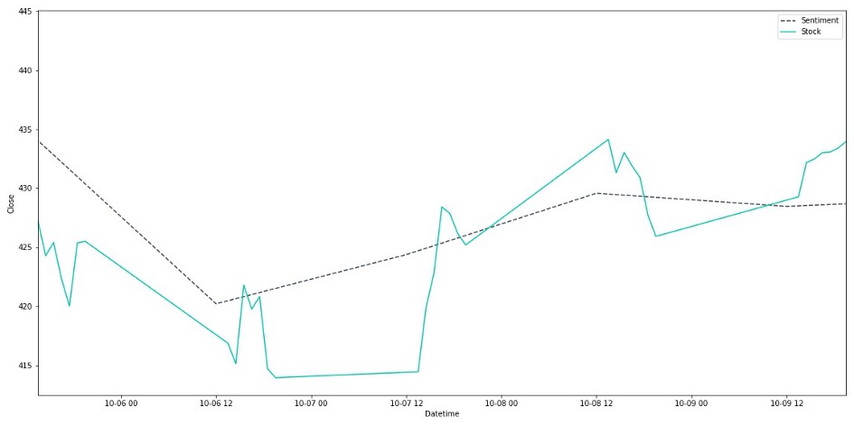
Our Flair model seems to work well, but do the tweets’ overall sentiment correlate with real stock price movements? By plotting Tesla tweets' sentiment alongside Tesla’s historical stock price performance, we can assess our approach’s potential viability.
TSLA Tweets
First, we need more data. Twitter offers the past seven days of data on their free API tier, so we will go back in 60-minute windows and extract ~100 tweets from within each of these windows.
To do this, we need to use v2 of the Twitter API — which is slightly different — but practically the same in functionality as v1. The full code, including API setup, is included below.
We tell the API our from-to datetime using the start_time and end_time parameters respectively, both require a datetime string in the format YYYY-MM-DDTHH:mm:ssZ.
from datetime import datetime, timedelta
import requests
import pandas as pd

# read bearer token for authentication
with open('bearer_token.txt') as fp:
    BEARER_TOKEN = fp.read()

# setup the API request
endpoint = 'https://api.twitter.com/2/tweets/search/recent'
headers = {'authorization': f'Bearer {BEARER_TOKEN}'}
params = {
    'query': '(tesla OR tsla OR elon musk) (lang:en)',
    'max_results': '100',
    'tweet.fields': 'created_at,lang'
}

dtformat = '%Y-%m-%dT%H:%M:%SZ'  # the date format string required by twitter

# we use this function to subtract 60 mins from our datetime string
def time_travel(now, mins):
    now = datetime.strptime(now, dtformat)
    back_in_time = now - timedelta(minutes=mins)
    return back_in_time.strftime(dtformat)

now = datetime.now()  # get the current datetime, this is our starting point
last_week = now - timedelta(days=7)  # datetime one week ago = the finish line
now = now.strftime(dtformat)  # convert now datetime to format for API

df = pd.DataFrame()  # initialize dataframe to store tweets

df = pd.DataFrame()  # initialize dataframe to store tweets
while True:
    if datetime.strptime(now, dtformat) < last_week:
        # if we have reached 7 days ago, break the loop
        break
    pre60 = time_travel(now, 60)  # get 60 minutes before 'now'
    # assign from and to datetime parameters for the API
    params['start_time'] = pre60
    params['end_time'] = now
    response = requests.get(api+search,
                            params=params,
                            headers=headers)  # send the request
    now = pre60  # move the window 60 minutes earlier
    # iteratively append our tweet data to our dataframe
    for tweet in response.json()['data']:
        row = get_data(tweet)  # we defined this function earlier
        df = df.append(row, ignore_index=True)
We write a function for subtracting 60 minutes from our datetime string — and integrate it into a loop that will run until we reach seven days into the past.
Inside this loop, we send our request for tweets within the 60-minute window — and then extract the information we want and append to our dataframe.
The result is a dataframe containing ~17K tweets containing the word ‘tesla’ from the past seven days.
API v2 allows us to include a specific language in our search query, so when adding (lang:en) to query we filter out anything that isn’t en (English) — leaving us with ~12K tweets.
TSLA Ticker
Next up, we need to extract our stock data from Yahoo Finance using the yfinance library — pip install yfinance if needed.
tsla = yf.Ticker("TSLA")tsla_stock = tsla.history(
    start=(data['created_at'].min()).strftime('%Y-%m-%d'),
    end=data['created_at'].max().strftime('%Y-%m-%d'),
    interval='60m'
).reset_index()
We initialize a Ticker object for TSLA, then use the history method to extract stock data between the min and max dates contained in our tweets data, with an interval of sixty minutes.
With a few transformations, we can overlay the average daily sentiment of our Tesla tweets above the stock price for Monday-Friday:
TSLA stock prices Monday-Friday. The sentiment (originally scored from -1 to +1 has been multiplied to accentuate +ve or -ve sentiment, and centered on the average stock price value for the week.
It’s clear that the Twitter sentiment and stock price are correlated during this week. Of course, a larger timespan would provide greater confidence — but this provides us with an initial positive outcome to investigate further.
That’s all for this introductory guide to sentiment analysis for stock prediction in Python. We’ve covered the basics of:
The Twitter API
Sentiment analysis with Flair
Yahoo Finance
Comparing our tweet sentiments against real stock data
There’s plenty more to learn to implement an effective predictive model based on sentiment, but it’s a great start.
Source: paper.li








Comments