In Machine Learning, the types of Learning can broadly be classified into 3 types: 1. Supervised Learning, 2. Unsupervised Learning and 3. Semi-supervised Learning. Algorithms belonging to the family of Unsupervised Learning have no variable to predict tied to the data. Instead of having an output, the data only has an input which would be multiple variables that describe the data. This is where clustering comes in.
Clustering is the task of grouping together a set of objects in a way that objects in the same cluster are more similar to each other than to objects in other clusters. Similarity is a metric that reflects the strength of relationship between two data objects. The distance is the most common metric used to measure similarity.
In this post I present k-means
The dataset used in this post is available from https://archive.ics.uci.edu
from Shinmoto Torres, R. L., Ranasinghe, D. C., Shi, Q., Sample, A. P. (2013, April). Sensor enabled wearable RFID technology for mitigating the risk of falls near beds. In 2013 IEEE International Conference on RFID (pp. 191–198). IEEE.
And the notebook is available in my github repo
The k-means is the most used algorithm in the business world for data clustering (unsupervised learning) thanks to its main advantages:
Good (or acceptable) accuracy and performance.
Its explicability, clusters can be easily explained to business people.
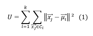
The K-means algorithm is not so complex. The wikipedia definition is : k-means clustering aims to partition n observations into k clusters, in which each observation belongs to the cluster with the nearest mean, serving as a prototype of the cluster. k-Means minimizes within-cluster variances (squared Euclidean distances), but not regular Euclidean distances, which would be the more difficult: the mean optimizes squared errors, whereas only the geometric median minimizes Euclidean distances.
Where ml is the mean of the elements inside the class Ci. In that case, the number of the clusters is fixed in advance and it represents the only parameter of the algorithm, the means being estimated recursively.
However, this algorithm has some drawbacks: the number of clusters K must be fixed beforehand, it converges to a local minimum and is not suitable for classes of non-convex structures and different sizes. But some pre-processing steps (i.e feature engineering) can help to cover this.
The first paragraph of the notebook, in the following lines shows how to load the data. Your data are located in the data/Datasets_Healthy_Older_People/dataset folder
import pandas as pd
import glob, ospathFiles = r’data/Datasets_Healthy_Older_People/dataset’
all_files = glob.glob(os.path.join(pathFiles, “*”))
li = []
for filename in all_files:
    df = pd.read_csv(filename, index_col=None, header= None, names=[‘timeSec’, ‘accFrontal’, ‘accVertical’, ‘accLateral’, ‘antennaID’, ‘rssi’, ‘phase’, ‘frequency’, ‘activity’])
    li.append(df)
dataAll = pd.concat(li, axis=0, ignore_index=True)
I will use scikit learn to perform the kmeans, more info at https://scikit-learn.org/stable/modules/generated/sklearn.cluster.KMeans.html
If you’re interested on implementing kmeans from scratch, you can find a post here https://medium.com/machine-learning-algorithms-from-scratch/k-means-clustering-from-scratch-in-python-1675d38eee42
Let’s divide the dataset into a train and a test set and remove some irrelevant columns such as antennaID, activity and frequency
import sklearn
dataAll1, dataAll2= sklearn.model_selection.train_test_split(dataAll, test_size=0.4, random_state=0)
dataAllPart = dataAll2.drop(['antennaID','activity', 'frequency'], axis=1)
Cluster evaluation: the silhouette score https://blog.floydhub.com/introduction-to-k-means-clustering-in-python-with-scikit-learn/
Before fixing the number of clusters, we can try a range of numbers to be sure that we are choosing the best number. There are two things to consider here:
If we have the ground truth labels (class information) of the data points available with us (which is not the case here) then we can make use of extrinsic methods like homogeneity score, completeness score and so on.
But if we do not have the ground truth labels of the data points, we will have to use the intrinsic methods like silhouette score which is based on the silhouette coefficient. We now study this evaluation metric in a bit more details.
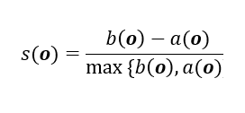
Let’s start with the equation for calculating the silhouette coefficient for a particular data point:
where,
- s(o) is the silhouette coefficient of the data point o
- a(o) is the average distance between o and all the other data points in the cluster to which o belongs
- b(o) is the minimum average distance from o to all clusters to which o does not belong
The value of the silhouette coefficient is between [-1, 1]. A score of 1 denotes the best meaning that the data point o is very compact within the cluster to which it belongs and far away from the other clusters. The worst value is -1. Values near 0 denote overlapping clusters.
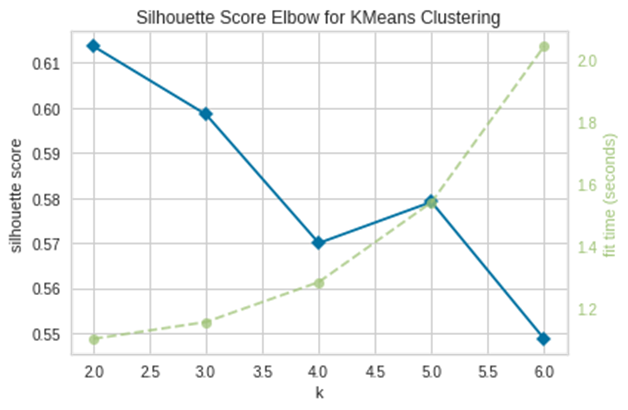
With scikit-learn, you can compute the silhouette coefficients for all the data points very easily using a range of number of clusters, here from 2 to 7:
from yellowbrick.cluster import KElbowVisualizer
kmeans = KMeans(random_state=120)
# Instantiate the KElbowVisualizer with the number of clusters and the metricvisualizer = KElbowVisualizer(kmeans, k=(2,7), metric='silhouette')
visualizer.fit(dataAllPart)
visualizer.poof()
The silouhette is higher for 2 classes meaning that 2 classes is the best number of classes to choose. Now, let’s build our model with 2 clusters.
# exploring the two classes
kmeans = KMeans(n_clusters=2)
dataAll21Class = kmeans.fit(dataAllPart)
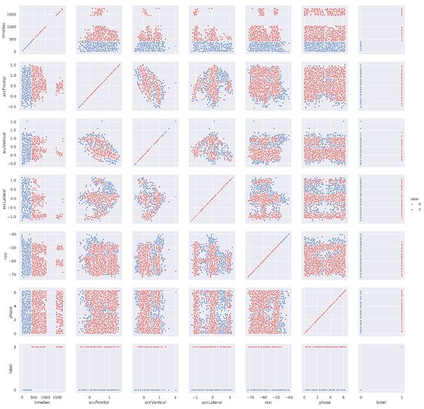
Let’s do a scatter matrix plot to check whether there are discriminating features or not.
import seaborn as sns
import pandas as pd
import matplotlib.pyplot as plt
from pylab import savefigsns.set()
dataAllPart['label'] = dataAll21Class.labels_.astype(str)
g = sns.PairGrid(dataAllPart, hue="label", hue_order=["0", "1"],
palette=["b", "r"],
hue_kws={"s": [20, 20], "marker": ["o", "o"]})
g.map(plt.scatter, linewidth=1, edgecolor="w")
g.add_legend()
plt.savefig('scatterMatrix.PNG', dpi=700)
We can see that timesec is the most discriminating feature since the two classes can be well distinguished whatever the axes used with the axis timesec in a scatter plot.
Another method that can be used to evaluate the clustering is the PCA. Principal component analysis (PCA) is a statistical procedure that uses an orthogonal transformation to convert a set of observations of possibly correlated variables (entities each of which takes on various numerical values) into a set of values of linearly uncorrelated variables called principal components. More info at https://en.wikipedia.org/wiki/Principal_component_analysis and https://scikit-learn.org/stable/modules/generated/sklearn.decomposition.PCA.html
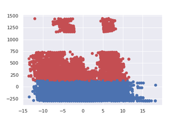
Here after the plot of the 2 first principal components:
from sklearn.decomposition import PCA
import matplotlib.pyplot as pltpcaGen = PCA(n_components=2).fit(dataAllPart)
pcaGen2Cmp = pcaGen.transform(dataAllPart)
plt.scatter(pcaGen2Cmp[:,0], pcaGen2Cmp[:,1], c=col, marker = ‘o’)
plt.savefig(“pca2.png”)
The figure shows that the points are well discriminated depending on the class. This prove that the clustering works fine.
These clusters can be used further for other purpose, example:
In Supervised leaning: we can divide timesec into two classes using the results of our clustering (labels being the clusters), train a supervised model on the labeled data.
This post is an introduction to the kmeans, I introduced the key concepts and the materials we need to build clusters using k-means when no prior information, no label is available. I did not discuss feature engineering including dealing with categorical features, scaling, etc. It was not the purpose of my present post.
In a future post, we will discuss those items.
SOURCE:paper.li




Comments